
View on GitHub

Open this notebook in GitHub to run it yourself

Classical Neural Networks

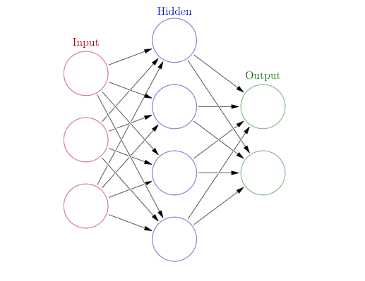
Neural networks is one of the major branches in machine learning, with wide use in applications and research. A neural network—or, more generally, a deep neural network—is a parametric function of a specific structure (inspired by neural networks in biology), which is trained to capture specific functionality. In its most basic form, a neural network for learning a function f:RNRM\vec{f}: \mathbb{R}^N\rightarrow \mathbb{R}^M looks as follows:
  1. There is an input vector of size NN (red circles in Fig. 1).
  2. Each entry of the input goes into a hidden layer of size KK, where each neuron (blue circles in Fig. 1) is defined with an “activation function” yk(w(1);x)y^{k}(\vec{w}^{(1)}; \vec{x}) for k=1,,Kk=1,\dots,K, and w(1)\vec{w}^{(1)} are parameters.
  3. The output of the hidden layer is sent to the output layer (green circles in Fig. 1) f~m(w(2);y)\tilde{f}^{m}(\vec{w}^{(2)};\vec{y}) for m=1,,Mm=1,\dots,M, and w(2)\vec{w}^{(2)} are parameters.
The output f~\vec{\tilde{f}} is thus a parametric function (in w(1),w(2)\vec{w}^{(1)},\,\vec{w}^{(2)}), which can be trained to capture the target function f\vec{f}. png
Deep neural networks are similar to the description above, having more than one hidden layer. This provides a more complex structure that can capture more complex functionalities.

Quantum Neural Networks

The idea of a quantum neural network refers to combining parametric circuits as a replacement for all or some of the classical layers in classical neural networks. The basic object in QNN is thus a quantum layer, which has a classical input and returns a classical output. The output is obtained by running a quantum program. A quantum layer is thus composed of three parts:
  1. A quantum part that encodes the input: This is a parametric quantum function for representing the entries of a single data point.
There are three canonical ways to encode a data vector of size NN: angle-encoding using NN qubits, dense angle-encoding using N/2\lceil N/2\rceil qubits, and amplitude-encoding using log2N\lceil\log_2N\rceil qubits.
  1. A quantum ansatz part: This is a parametric quantum function, whose parameters are trained as the weights in classical layers.
  2. A postprocess classical part, for returning an output classical vector.
The integration of quantum layers in classical neural networks may offer reduction in resources for a given functionality, as the network (or part of it) is expressed via the Hilbert space, providing different expressibility compared to classical networks. This notebook demonstrates QNN by treating a specific function—the subset majority—for which we construct, train, and verify a hybrid classical-quantum neural network. The notebook assumes familiarity with Classiq and NN with PyTorch. See the QML guide with Classiq.

Example: Hybrid Neural Network for the Subset Majority Function

For an integer NN and a given subset of indices S{0,1,,N}S \subset \{0,1,\dots,N\} we define the subset majority function, MS:{0,1}×N{0,1}M_{S}:\{0,1\}^{\times N}\rightarrow \{0,1\} that acts on binary strings of size NN as follows: it returns 1 if the number of ones within the substring according to SS is larger than S//2|S|//2, and 0 otherwise, MS(b)={1if jSbj>S//2,0otherwiseM_S(\vec{b}) = \left\{ \begin{array}{l l } 1 & \text{if } \sum_{j\in S} b_{j}>|S|//2, \\ 0 & \text{otherwise} \end{array} \right . For example, we consider N=7N=7 and S={0,1,4}S=\{0,1,4\}:
  • The string 0101110 corresponds to the substring 011, for which the number of ones is 2(>1). Therefore, MS(0101110)=1M_S(0101110)=1.
  • The string 0011111 corresponds to the substring 001, for which the number of ones is 1(=1). Therefore, MS(0101110)=0M_S(0101110)=0.

Generating Data for a Specific Example

Let us consider a specific example for our demonstration. We choose N=10N=10 and generate all possible data of 2N2^N bit strings. We also take a specific subset S={1,3,4,6,7,9}S=\{1, 3, 4, 6, 7, 9\}.
!pip install -qq -U "classiq[qml]"

import random

import numpy as np

np.random.seed(0)
random.seed(1)

STRING_LEN = 10
majority_data = [
    [int(d) for d in np.binary_repr(k, STRING_LEN)] for k in range(2**STRING_LEN)
]
random.shuffle(majority_data)  # shuffling the data

SUBSET_INDICES = [1, 3, 4, 6, 7, 9]
subset_indicator = np.zeros(STRING_LEN)
subset_indicator[SUBSET_INDICES] = 1

majority = (majority_data @ subset_indicator > len(SUBSET_INDICES) // 2) * 1
labels = [[l] for l in majority]
We choose data for training and data for verification, and define the batch size for the corresponding data loaders:
TRAINING_SIZE = 340
TEST_SIZE = 512

training_data = majority_data[0:TRAINING_SIZE]
training_labels = labels[0:TRAINING_SIZE]
test_data = majority_data[TRAINING_SIZE : TRAINING_SIZE + TEST_SIZE]
test_labels = labels[TRAINING_SIZE : TRAINING_SIZE + TEST_SIZE]

BATCH_SIZE = 64

import numpy as np
import torch
from torch.utils.data import DataLoader, TensorDataset

training_dataset = TensorDataset(
    torch.Tensor(training_data), torch.Tensor(training_labels)
)  # create dataset
training_dataloader = DataLoader(
    training_dataset, batch_size=BATCH_SIZE, shuffle=True, drop_last=False
)  # create dataloader

test_dataset = TensorDataset(
    torch.Tensor(test_data), torch.Tensor(test_labels)
)  # create your dataset
test_dataloader = DataLoader(
    test_dataset, batch_size=BATCH_SIZE, shuffle=True, drop_last=False
)  # create your dataloader

Constructing a Hybrid Network

We build the following hybrid neural network: Data flattening \rightarrow A classical linear layer of size 10 to 4 with Tanh activation \rightarrow A qlayer of size 4 to 2 \rightarrow a classical linear layer of size 2 to 1 with ReLU activation. The classical layers can be defined with PyTorch built-in functions. The quantum layer is constructed with (1) a dense angle-encoding function (2) a simple ansatz with RY and RZZ rotations (3) a postprocess that is based on a measurement per qubit

The Quantum Layer

from classiq import *
from classiq.applications.qnn.types import SavedResult
from classiq.execution import ExecutionPreferences, execute_qnn


@qfunc
def my_ansatz(weights: CArray[CReal], qbv: QArray) -> None:
    """
    Gets a quantum variable of $m$ qubits, and applies RY gate on each qubit and RZZ gate on each pair of qubits
    in a linear connectivity.

The classical array weights represents the $2m-1$ parametric rotations.
    """
    repeat(
        count=qbv.len,
        iteration=lambda index: RY(weights[index], qbv[index]),
    )
    repeat(
        count=qbv.len - 1,
        iteration=lambda index: RZZ(weights[qbv.len + index], qbv[index : index + 2]),
    )

QLAYER_SIZE = 4
num_qubits = int(np.ceil(QLAYER_SIZE / 2))
num_weights = 2 * num_qubits - 1
NUM_SHOTS = 4096


@qfunc
def main(
    input: CArray[CReal, QLAYER_SIZE],
    weight: CArray[CReal, num_weights],
    result: Output[QArray],
) -> None:
    """
    The quantum part of the quantum layer.

The prefix for the data loading parameters must be set to `input_` or `i_`.

The prefix for the ansatz parameters must be set to `weights_` or `weight`
    """
    encode_on_bloch(input, result)
    my_ansatz(weights=weight, qbv=result)


qmod = create_model(
    main, execution_preferences=ExecutionPreferences(num_shots=NUM_SHOTS)
)
qprog = synthesize(qmod)
show(qprog)
Output:

Quantum program link: https://platform.classiq.io/circuit/32pQqOSulTv1Qvssd71mPgf4btU
  

def my_post_process(result: SavedResult, num_qubits, num_shots) -> torch.Tensor:
    """
    Classical postprocess function.

Gets the histogram after execution and returns a vector $\vec{y}$,
    where $y_i$ is the probability of measuring 1 on the $i$-th qubit.
    """
    res = result.value
    yvec = [
        (res.counts_of_qubits(k)["1"] if "1" in res.counts_of_qubits(k) else 0)
        / num_shots
        for k in range(num_qubits)
    ]

    return torch.tensor(yvec)

The Full Hybrid Network

Now, we can define the full network.
import torch.nn as nn

from classiq.applications.qnn import QLayer


def create_net(*args, **kwargs) -> nn.Module:
    class Net(nn.Module):
        def __init__(self, *args, **kwargs):
            super().__init__()
            self.flatten = nn.Flatten()
            self.linear_1 = nn.Linear(STRING_LEN, 4)
            self.activation_1 = nn.Tanh()
            self.linear_2 = nn.Linear(2, 1)
            self.activation_2 = nn.ReLU()

            self.qlayer = QLayer(
                qprog,
                execute_qnn,
                post_process=lambda res: my_post_process(
                    res, num_qubits=num_qubits, num_shots=NUM_SHOTS
                ),
                *args,
                **kwargs,
            )

        def forward(self, x):
            x = self.flatten(x)
            x = self.linear_1(x)
            x = self.activation_1(x)
            x = self.qlayer(x)  # 4 to 2
            x = self.linear_2(x)  # 2 to 1
            x = self.activation_2(x)
            return x

    return Net(*args, **kwargs)


my_network = create_net()

Training and Verifying the Networks

We define some hyperparameters such as loss function and optimization method, and a training function:
import torch.nn as nn
import torch.optim as optim

LEARNING_RATE = 0.05

# choosing our loss function
loss_func = nn.MSELoss()

# choosing our optimizer
optimizer = optim.SGD(my_network.parameters(), lr=LEARNING_RATE)
Next, we define a train function:
import time as time

from torch.utils.data import DataLoader


def train(
    network: nn.Module,
    data_loader: DataLoader,
    loss_func: nn.modules.loss._Loss,
    optimizer: optim.Optimizer,
    epoch: int = 20,
) -> None:
    for index in range(epoch):
        start = time.time()
        for data, label in data_loader:

            optimizer.zero_grad()
            output = network(data)
            loss = loss_func(output, label.type(output.dtype))
            loss.backward()

            optimizer.step()

        print(index, f"\tloss = {loss.item()}", "time", time.time() - start)
We also define a validation function, check_accuracy, which tests a trained network on new data:
from torch import Tensor


def get_correctly_guessed_labels_function(
    model: nn.Module, data: Tensor, labels: Tensor
) -> int:
    predictions = model(data)
    list_of_predictions = [
        round(prediction.type(torch.float).item()) for prediction in predictions
    ]
    correct = sum(
        [
            list_of_predictions[k] == labels.flatten().tolist()[k]
            for k in range(len(predictions))
        ]
    )
    return correct


def _get_amount_of_labels(labels: Tensor) -> int:
    # the first dimension of `labels` is `batch_size`
    return labels.size(0)


def check_accuracy(
    network: nn.Module,
    data_loader: DataLoader,
    should_print: bool = True,
) -> float:
    num_correct = 0
    total = 0

    network.eval()

    with torch.no_grad():
        for data, labels in data_loader:
            num_correct += get_correctly_guessed_labels_function(network, data, labels)
            total += _get_amount_of_labels(labels)

    accuracy = float(num_correct) / float(total)

    if should_print:
        print(f"Test accuracy of the model: {accuracy*100:.2f}%")
        print(f"num correct: {num_correct}, total: {total}")

    return accuracy

Training and Verifying the Network

For convenience, we load a pre-trained model and set the epoch size to
  1. Training a network takes around 30 epochs.
# comment out for training
my_network.load_state_dict(torch.load("trained_model.pth"))
num_epoch = 1
# uncomment out for training
# epoch=30

data_loader = training_dataloader
train(my_network, training_dataloader, loss_func, optimizer, epoch=num_epoch)
Output:
0 	loss = 0.09676678478717804 time 169.12708473205566
  

accuracy = check_accuracy(my_network, test_dataloader)
Output:

Test accuracy of the model: 97.07%
  num correct: 497, total: 512